Archive
Faster turtles
Using the Python Imaging Library I’ve created a faster alternative to the turtle.py module. It takes only a few seconds to draw images that were taking several minutes with turtle.py.
There are a few downsides to this approach I suppose:
- There is no on-screen animation of the image being created which is useful tool when teaching turtle graphics — only a finished image is created.
- Output is a raster image, not a nice svg or eps file.
On the up side:
- Super fast
- Antialiased
- All Python Imaging Library tools and methods also available.
- At the moment is largely compatible with the turtle.py module
Who knows… once I’ve got the code into a more finished state I may share my fast-turtle module with the world.
Here’s a nice animation that I created with my aforementioned fast turtle module:
Turtle.py
Python comes with a turtle graphics module right there in the standard library. A new and improved version was introduced with Python 2.6, and it is quite good. I think its real strength could be in the initial stages of teaching kids to program in Python.
For my use I found two major drawbacks. First, there is no built-in way to export your drawing to an image file (taking a screenshot is the solution I’ve been using). More importantly, the turtle drawing is intolerable slow for complex images.
I did manage to create this rather nice recursive tree:

(The leaves are dead turtles)
Nevertheless I think I will concentrate on some other turtle graphics implementation for now. After all, I already program in Python so I won’t be learning anything new there. Also did I mention slow? So slow.
I would be interested in learning UCBLogo as the language itself would be interesting for me to learn (A far more turtle-y Lisp dialect). Also from my initial tests it seems to be so much faster than turtle.py. However it also has limited capacity to save drawings as images (only eps output with no filled shapes 😦 ). The output window also appears buggy on my Ubuntu Linux system… The image in the window does not refresh after being obscured or minimised, which pretty much makes it useless to me until this issue has been addressed. I figured out that turning on window compositing fixes this somewhat. The output is no longer deleted after the output window is obscured by another window. If you minimise or resize the window the image disappears, but seems to come back most of the time if you type “REFRESH” into the Logo session.
Talking Python
The following was a small amusement that I put together for my 5 year old daughter. It must have made quite the impression on her as she has informed me that she wants to be a “horse programmer” when she grows up.
This program relies on another program called “espeak” which should be present on most Linux systems. This is a command line tool which takes text and converts it to speech. If you are using a Mac you could adapt the program to use the command “say” which does the same thing (the command line arguments are bound to be different though). Windows doesn’t include such a tool, because Microsoft just doesn’t love you, however Google turned up this result when I searched for “Windows command line speech”.
Apart from that you will see a few Python constructs which may be interesting to Python newbies, such as calling another program from within your Python script, and generating random silly sentences.
Note that it also uses the new style of string formatting so you will need at least Python version 2.6.
#! /usr/bin/python

import subprocess
import random

def say(sentence):
    speed = "-s " + str(random.randrange(120, 200))
    pitch = "-p " + str(random.randrange(100))
    subprocess.call(["espeak", speed, pitch, sentence])

sentences = [
    "Hello {name}.",
    "{name}? What a {adjective} name!",
    "Congratulations, {name}! You have won a {noun}!",
    "Excuse me {name}. Have you seen my {adjective} {noun}?",
    "Hello {name}. Are you going to Wellington Zoo soon {name}?",
    "What is your name {name}? Oh, that's right, silly me. Your name is {name}!",
    "{name}! Your {adjective} {noun} is {verb}ing! {adverb} grab a {noun2}, {name}!",
    "What is your favourite {noun}, {name}? Is it the {adjective} one?",
    "Quickly quickly {name}! No and Yes!",
    "Where's your mummy {name}? Is she {verb}ing today?",
    "That's what I said {name}",
    "What are you doing {name}? Are you {adverb} {verb}ing? Do you think that's a good idea?",
    "{noun}s are fun. Don't you think so {name}?",
    "Red alert. We go beserk. No {name} moves, no {name} gets hurt.",
    "Please {name}. May we go to the {noun} shop?",
    "Happy birthday to you. Happy Birthday to you."
    " Happy birthday dear {name}. Happy birthday to you!",
    "This is a shout out to {name}. Keep it real homey.",
    "Last night I had the strangest dream. {name} was {adverb} riding on "
    "a {adjective} {noun}, being chased by a thousand {adjective2} {noun2}s. "
    "Luckily, the {noun} was just too {adjective} for the {noun2}",
    "{name} is a good reader!",
    "Time for bed {name}. Go on... off you go!",
    "Make me a {noun} {name}, as fast as you can! I would like a {adjective} one please!",
    "Who ate all of my cake? {name}, was it you?",
    "I'm lost {name}! Can you tell me where I am?",
    "Do you like the circus {name}?",
    "This is the {adjective}est {noun} that I have ever seen. It is even more {adjective} than "
    "that {noun2} that I saw yesterday. Although, to be honest, that {noun2} "
    "was probably more {adjective2} than {adjective}",
    "I just saw a {adjective} {noun} {adverb} {verb}ing a {adjective2} {noun2}.",
    "Never let a {noun} {verb} more than once a day, otherwise it may {adverb} turn "
    "into a {noun2}",

    ]

nouns = [
    "pony",
    "horse",
    "cheesecake",
    "muffin",
    "dragon",
    "car",
    "DVD",
    "Computer",
    "Rollercoaster",
    "Hamburger",
    "Chestnut Park",
    "Cat",
    "dog",
    "TV",
    "soccer ball",
    "sandwich",
    "X box",
    "house",
    "bus",
    "van",
    ]

adjectives = [
    "silly",
    "fast",
    "brown",
    "pink",
    "yellow",
    "blue",
    "purple",
    "golden",
    "funky",
    "red",
    "bouncy",
    "pretend",
    "angry",
    "madd",
    "sadd",
    "badd",
    "grumpy",
    "stupid",
    "awesome",
    "ridiculous",
    "dubious",
    "dodgy",
    "flightless",
    "sleepy",
    "antogonistic",
    ]

verbs = [
    "talk",
    "ignore",
    "runn",
    "grump",
    "riyd",
    "gallop",
    "program",
    "slide",
    "gasp",
    "shout",
    "jump",
    "read",
    "play"
    "dodge",
    "crawl",
    "whisper",
    "hiyd",
    "smell",
    "sink",
    ]

adverbs = [
    "quickly",
    "suddenly",
    "slowly",
    "agrily",
    "Greedily",
    "happily",
    "mostly",
    "rapidly",
    "forcefully",
    "woodenly",
    "passionately",
    ]

n = ""
while True:
    n = raw_input("What is your name? ")
    if not n: break
    #[say(word) for word in random.choice(sentences).format(name=n).split()]
    for i in range(3):
        say(random.choice(sentences).format(name=n,
                                            noun = random.choice(nouns),
                                            noun2 = random.choice(nouns),
                                            verb = random.choice(verbs),
                                            adverb = random.choice(adverbs),
                                            adjective = random.choice(adjectives),
                                            adjective2 = random.choice(adjectives),
                                            ))
Making a rogue-like game with libtcod
Well I haven’t yet made a roguelike game, but I have completed a short tutorial on using the libtcod library.

Trapped in a lonely dungeon. Wait... who's that?!
Libtcod is a library with wrappers available for numerous programming languages which aids in the creation of roguelike games. I happen to be using the Python wrapper.
It provides a special true-colour console with plenty of neat tricks like customizable fonts, blitting of images and off screen drawing areas. These provide the potential for some stunning visuals that still have a blocky, old-school, feel.
While I’m sure these facts alone would make it useful for a great many styles of game, libtcod also provides numerous helpful toolkits which, for the most part, are aimed at roguelike developers.
Basically all of the standard routines that you would otherwise need to figure out for yourself before you can start designing your unique game. These include:
- Field of view toolkit. What can you see in the dungeon… where does your torchlight fall?
- Path finding toolkit. Compute the path from A to Z in your dungeon.
- Keyboard and mouse support
- BSP dungeon generation toolkit. Tweak the parameters for dungeons, towns, forests or whatever.
Plus a few more neat features you may not have ever imagined you would need for a roguelike:
- BMP and PNG support
- Heightmap toolkit 😯
- Perlin noise support. Hmmm… ocean anyone?
- Random number and compression toolkits
It’s probably important to note that you can use any or all of the toolkits that you choose… If you would prefer to implement your own dungeon generator for example, that’s fine too. In fact there is still plenty of work still to be done as a game developer. For instance, libtcod won’t implement the monster AI or combat for you (yet).
Lately I’ve been focusing on learning C++, and if I’m to learn one new language a year (which seems a reasonable goal) then this is certainly the year of C++. However, I would also like to have fun with a language that I already know well (ie. Python), and this is where I see libtcod fitting in. My verdict so far is that I like this library and I think I could have a lot of fun tinkering with it.
I’ll post my game here when it’s awesome 😀
Crikey, I nearly forgot! The tutorial that I was blathering on about at the top of this post is here. At the time of writing this only the first part has been written, but that is enough to create the explorable dungeon level seen in the screenshot above. Here’s hoping that the authors finish the remainder of the tutorial sometime soon.
SPOJ
So I’m hooked on SPOJ again. For this burst of enthusiasm I’m using C++, both to increase my skills and to clean up some of the problems that my Python solutions could not solve in the given time limit.
Of course this process does not produce many (any) pretty pictures, therefore not much content for this fledgling blog.
Still, maybe I’ll discover some sort of algorithm or something.
I was rather proud of myself for figuring out the relationship between the curved perimeter of a semi-circle and its area (yes, pretty advanced stuff, I know :-P). Where “p” is the curved part of the semi-circle’s perimeter, and “A” is the area:

I don’t want to give away exactly which problem this was for, but it would sure be useful if you needed to enclose the maximal space possible against an infinitely long wall by adding a fence of a given length and arbitrary shape which touches the wall at exactly two points.. *cough* 😉
See Plus Plus
These Buddhabrot scripts can sure be processor intensive. I would be better off programming them in C or C++, much as I do love Python. They are rather trivial, so it shouldn’t be too difficult.
One purpose of this blog is to openly record my musings of the various things that I think I ought to do—in the hope that I may remember to actually do them. This is but one such open musing.
Buddhabrot Chromatica
In my previous post on Buddhabrots I demonstrated that different iteration or “bail-out” levels can produce different looking Buddhabrots. Buddhabrot discoverer Melinda Green also described the method of mapping differently-iterated Buddhabrots to the different channels of an RGB image. This can result in strikingly “Nebulous” images, reminiscent of those famous images from the Hubble space telescope.
Obviously this was the next thing I had to try.

3000r, 1500g, 500b. Channels normalized individually.
This image uses 3000 iterations on the red channel, 1500 on the green channel, and 500 on the blue channel. I have normalized the channels individually which seems to favor the channel with the least iterations.

3000r, 1500g, 500b. Channels normalized together.
This images uses the same configuration of iterations per channel as the last. This seems to favor the channel with the most iterations.
It strikes me that both of these approaches are rather arbitrary. The best solution would be to combine the channels in a decent image editing program and adjust the levels of each until the result is visually appealing (These images had their channels combined at creation time in Python). Unfortunately GIMP is not the decent image editing program I’m looking for. CinePaint, however, seems perfect for this job.

1000r, 200g, 100b. Adjusted in CinePaint
“To infinity… and beyond!”
1000 iterations red, 200 green, 100 blue. Adjusted to Hubbletastic perfection. Thanks CinePaint!
The next step is probably to render some super-big color images.
The Buddhabrot
The Buddhabrot is closely related to the Mandelbrot set. For both, you would calculate the orbit of z under the dynamic 
When rendering the Mandelbrot set we are chiefly concerned with values of c corresponding to pixels in our final image. We check which values of c cause the path of z to enter an orbit around the origin, and which values of c cause z to fly off to infinity (and how quickly). Pixels are then coloured accordingly.
For a Buddhabrot, the value of c is less important. Instead, the frequency with which the orbiting point z visits various pixels is recorded — lighter pixels have received a higher frequency of visits from z. While values of c are chosen at random, the classic Buddhabrot uses only those values of c which will cause z to escape to infinity (non Mandelbrot-set points). I think of this process as being a cross between a Mandelbrot set and a strange attractor.
Here is my first attempt at rendering a Buddhabrot using a program I wrote in Python:

This is a 100 iteration image This means that, when checking to see if an orbiting z point is escaping to infinity, we bail-out after 100 iterations and assume all remaining points are within the Mandelbrot set (their orbits are not used in the Buddhabrot). More iterations means more of the kind of orbit that take longer to escape.
It turns out that adjusting this ‘bail-out’ level can have a dramatic impact on the resulting image. For example, here is a 1000 iteration image:

We can see that higher bail-out values result in finer details.
Finally, a 5000 iteration image (click for super-high-res):

Here is the Python code in full, with gratuitous comments and print statements included — remember that you will need PyPng and Numpy to run this code.
#! /usr/bin/python
import png
import numpy as np
from random import random

def c_set(num_samples, iterations):
    # return a sampling of complex points outside of the mset

    # Allocate an array to store our non-mset points as we find them.
    non_msets = np.zeros(num_samples, dtype=np.complex128)
    non_msets_found = 0

    # create an array of random complex numbers (our 'c' points)
    c = (np.random.random(num_samples)*4-2 + \
        (np.random.random(num_samples)*4-2)*1j)

    # Optimizations: most of the mset points lie within the
    # within the cardioid or in the period-2 bulb. (The two most
    # prominant shapes in the mandelbrot set. We can eliminate these
    # from our search straight away and save alot of time.
    # see: http://en.wikipedia.org/wiki/Mandelbrot_set#Optimizations

    print "%d random c points chosen" % len(c)
    # First elimnate points within the cardioid
    p = (((c.real-0.25)**2) + (c.imag**2))**.5
    c = c[c.real > p- (2*p**2) + 0.25]
    print "%d left after filtering the cardioid" % len(c)

    # Next eliminate points within the period-2 bulb
    c = c[((c.real+1)**2) + (c.imag**2) > 0.0625]
    print "%d left after filtering the period-2 bulb" % len(c)

    # optimizations done.. time to do the escape time algorithm.
    # Use these c-points as the initial 'z' points.
    # (saves one iteration over starting from origin)
    z = np.copy(c)

    for i in range(iterations):
        # apply mandelbrot dynamic
        z = z ** 2 + c

        # collect the c points that have escaped
        mask = abs(z) < 2
        new_non_msets = c[mask == False]
        non_msets[non_msets_found:non_msets_found+len(new_non_msets)]\
                  = new_non_msets
        non_msets_found += len(new_non_msets)

        # then shed those points from our test set before continuing.
        c = c[mask]
        z = z[mask]

        print "iteration %d: %d points have escaped!"\
        % (i + 1, len(new_non_msets))

    # return only the points that are not in the mset
    return non_msets[:non_msets_found]

def buddhabrot(c, size):
    # initialise an empty array to store the results
    img_array = np.zeros([size, size], int)

    # use these c-points as the initial 'z' points.
    z = np.copy(c)

    while(len(z)):

        print "%d orbits in play" % len(z)
        # translate z points into image coordinates
        x = np.array((z.real + 2.) / 4 * size, int)
        y = np.array((z.imag + 2.) / 4 * size, int)

        # add value to all occupied pixels
        img_array[x, y] += 1

        # apply mandelbrot dynamic
        z = z ** 2 + c

        # shed the points that have escaped
        mask = abs(z) < 2
        c = c[mask]
        z = z[mask]

    return img_array

if __name__ == "__main__":

    size = 400 # size of final image
    iterations = 200 # bailout value -- higher means more details
    samples = 10000000 # number of random c points chosen

    img_array = np.zeros([size, size], int)

    i = 0

    while True:

        print "get c set..."
        c = c_set(samples, iterations)
        print "%d non-mset c points found." % len(c)

        print "render buddha..."
        img_array += buddhabrot(c, size)

        print "adjust levels..."
        e_img_array = np.array(img_array/float(img_array.max())*((2**16)-1), int)

        print "saving buddhabrot_n_%di_%03d.png" % (iterations,i)
        # save to final render to png file
        imgWriter = png.Writer(size, size, greyscale=True, alpha=False, bitdepth=16)
        f = open("buddhabrot_n_%di_%03d.png" % (iterations,i), "wb")
        imgWriter.write(f, e_img_array)
        f.close()

        print "Done."
        i += 1
Numpy and the Mandelbrot Set
I’ve now rendered my first Mandelbrot set, which was unexpectedly easy.
The concept of how to render the Mandelbrot set really only crystallized in my mind when I saw the following image:

Complex Mandelbrot Illustration by Kan8eDie
This is in fact the lead illustration on Wikipedia’s Complex Number page (redistributed here under the Creative Commons Attribution ShareAlike 3.0 License). To my mind it provides a clearer demonstration of how the Mandelbrot set is formed than anything on Wikipedia’s Mandelbrot Set page.
Points in the Mandelbrot set are just complex numbers with the real and imaginary parts mapped to the x and y axis respectively (known as the complex plane or Argand diagram). A simple repeated calculation then determines whether a given point is part of the Mandelbrot set:

That is, starting with z at the origin, square z and add a complex constant c. The process of squaring the result and then adding the constant c is repeated until it is apparent that the the point z is either orbiting close to the origin (therefore indicating that the constant c is a member of the Mandelbrot set) or diverging to infinity (c is not a part of the Mandelbrot set). Simply plot on the complex plane which values of c are included in this set and the classic Mandelbrot set fractal should appear before your eyes as if by magic.
The procedures for such operations as multiplying and adding complex numbers are quite straight forward. You can get the gist of the kind of things that may happen when multiplying by a complex number by examining the image above (The point rotates on the complex plane). However, it is even easier when programming in a language such as Python which has built-in support for complex numbers.
Consider the following interactive Python session
>>> a = (2 + 3j)
>>> b = (1 - 8j)
>>> a * b
(26-13j)
>>> z = a**2 + a
>>> z = z**2 + a
>>> z
(-214-87j)
The first four lines assign two complex numbers a and b and then display their product. The next four lines show exactly the kind of calculation one would need to do to find the Mandelbrot set. Easy.
Another useful tool is Python’s built in abs function. For real numbers this returns the absolute value of that number. For a complex number however, abs returns the modulus of the number. That is, it’s distance from the origin on the complex plane.
Abs is extremely useful in calculating the Mandelbrot set, as any orbit which strays more than distance 2 from the origin is known to be not part of the Mandelbrot set. Further testing of the point c is unnecessary and the next point can then be tested.

My first Mandelbrot
My first Python script for rendering the Mandelbrot set simply looped through each pixel in the image one at a time. Each pixel is assigned a complex number from a 4 x 4 grid. That is, a number in the square bounded by (-2 – 2j) and (2 + 2j). For each pixel I then applied the “square and add a constant” dynamic for a certain number of iterations to determine if it is a member of the Mandelbrot set.
This technique works, but is quite slow. Here is the code in its entirety:
#! /usr/bin/python
import png
import numpy as np
import datetime

def mandelbrot_set(size, exit_limit):

    # initialize array
    img_array = np.zeros([size, size], int)

    for y in range(size):
        for x  in range(size):

            c = complex(x / float(size) * 4 - 2,
                        y / float(size) * 4 - 2)
            z = c

            for i in range(exit_limit):
                z = (z**2) + c
                img_array[y, x] += 1

                if abs(z) > 2:
                    # z is escaping to infinity, so point is not in set
                    break
            else:
                # if loop is exausted, point is inside the set
                img_array[y, x] = 0
    return img_array

if __name__ == "__main__":

    start = datetime.datetime.now()

    # size of final image:
    size = 1600

    # after this many iterations, point is assumed to be within the
    # mandelbrot set:
    exit_limit = 64

    imgWriter = png.Writer(size, size,
                           greyscale=True, alpha=False, bitdepth=16)

    img_array = mandelbrot_set(size, exit_limit)

    # normalise array (16 bit range)
    img_array = np.array(img_array/float(img_array.max())*(2**16), int)

    # save to final render to png file
    f = open("mandelbrot.png", "wb")
    imgWriter.write(f, img_array)
    f.close()

    print datetime.datetime.now()-start
    print "Done."
If you are wondering where the different shades of color come from, It it simply that the lighter shades take more iterations for z to escape to a distance of 2 from the origin. The black pixels in the middle of the shape indicate that z does not escape.
Now how could I speed this program up? Looping through each pixel is inherently slow. I decided to try again, this time using a Numpy array of complex numbers (yes, complex numbers are a valid data-type in Numpy!). Now I no longer need to loop through the pixel of my image, only through the iterations of the “square and add a constant” dynamic.
This reduces the rendering time to about a third of that needed for the pixel-looping solution above! The only drawback seems to be that this method can use a lot of memory while its running. This is a problem if you want to create a very large image. For example, attempting to render a 3200 x 3200 image results in an error on my computer just due to the vast size of the complex number array that is required. That problem could easily be solved by rendering the image in several smaller chunks that are more RAM friendly. The image array is okay at that size (it’s just integers after all), so there would be no need to be manually stitching the pieces together afterwards!
Here is the code for my Numpy solution:
import numpy as np
import png
from datetime import datetime

start = datetime.now()

size = 800
iterations = 63

# turn range(0, size**2) into an array of complex values encompassing the render area
complex_val = lambda p: complex(p%size/float(size)*4-2, p/size/float(size)*4-2)
c = np.array([complex_val(p) for p in range(size**2)])\
              .reshape(size, size)

# This array is used to mask out values that have already escaped:
operation_mask = np.ones((size, size), np.bool)

# This will become the final image:
iteration_array = np.zeros((size, size), np.int32)

# our starting "z" values. Note I don't start at '0' because 0**2 + c is clearly c.
z = np.copy(c)

for x in range(iterations):
    print "iteration %d" % x

    z[operation_mask] = (z[operation_mask]**2) + c[operation_mask]
    iteration_array[operation_mask] += 1

    # remove values form the "operation mask" if their calculation has diverged
    operation_mask[operation_mask] = np.absolute(z[operation_mask]) < 2

# finally, paint points in the mandelbrot set black.
iteration_array[operation_mask] = 0

imgwriter = png.Writer(size, size, greyscale=True, alpha=False, bitdepth=8)
f = open('m.png', 'wb')
imgwriter.write(f, iteration_array)
f.close()

print datetime.now() - start
Where to from here? There a few things I could try next:
- Smooth coloration – get rid of the color banding
- Interactive zooming and exploration, using PyGame perhaps
- Render the Buddhabrot attractor, because that looks cool
- More speed optimizations.
Smarter Colors

Clam Shell from Space
Gradient mapping can produce nice results, but I got to wondering if there was another way. Perhaps there is a way for a strange attractor to produce it’s own color scheme. As there are often many intricate and overlapping elements in these images, I needed some unique characteristic that will identify these separate elements and decide their color.
The strange attractors are generated by a single point jumping around the place according to a set of formulas:

It occurs that if the (x, y) position of any given point in the strange attractor is determined by its “parent” point — the (x, y) values that are passed into the f and g formulas.
So, one unique characteristic of any given point in a strange attractor is the location of its parent point. This is the idea I used to colorize these new images.
Take a look at this snippet of Python code and you will see how the color of the next pixel is calculated before the new x and y values are calculated:
# determine the color of the next pixel based on current x position
color = hsv_to_rgb(x+trap_size, .8, 1)

# calculate the new x, y based on the old x, y
x, y = (a*(x**2) + b*x*y + c*(y**2) + d*x + e*y + f,
        g*(x**2) + h*x*y + i*(y**2) + j*x + k*y + l)

# translate floats, x, y into array indices
px = int((x+trap_size)*(size/(trap_size*2)))
py = int((y+trap_size)*(size/(trap_size*2)))

# add some colour to the corresponding pixel
img_array[px, py, :] += np.array(color)
This code uses a useful module from the Python standard library, colorsys, which provides functions for converting between color models.
This method achieved the goal of applying different colors to distinct overlapping elements. This a a feat which cannot be achieve by mapping a gradient to a greyscale image.
Here a few more images which demonstrate this effect (click to enlarge):
-

- Clam Shell from Space