Archive
Smarter Colors

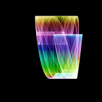
Clam Shell from Space
Gradient mapping can produce nice results, but I got to wondering if there was another way. Perhaps there is a way for a strange attractor to produce it’s own color scheme. As there are often many intricate and overlapping elements in these images, I needed some unique characteristic that will identify these separate elements and decide their color.
The strange attractors are generated by a single point jumping around the place according to a set of formulas:

It occurs that if the (x, y) position of any given point in the strange attractor is determined by its “parent” point — the (x, y) values that are passed into the f and g formulas.
So, one unique characteristic of any given point in a strange attractor is the location of its parent point. This is the idea I used to colorize these new images.
Take a look at this snippet of Python code and you will see how the color of the next pixel is calculated before the new x and y values are calculated:
# determine the color of the next pixel based on current x position
color = hsv_to_rgb(x+trap_size, .8, 1)

# calculate the new x, y based on the old x, y
x, y = (a*(x**2) + b*x*y + c*(y**2) + d*x + e*y + f,
        g*(x**2) + h*x*y + i*(y**2) + j*x + k*y + l)

# translate floats, x, y into array indices
px = int((x+trap_size)*(size/(trap_size*2)))
py = int((y+trap_size)*(size/(trap_size*2)))

# add some colour to the corresponding pixel
img_array[px, py, :] += np.array(color)
This code uses a useful module from the Python standard library, colorsys, which provides functions for converting between color models.
This method achieved the goal of applying different colors to distinct overlapping elements. This a a feat which cannot be achieve by mapping a gradient to a greyscale image.
Here a few more images which demonstrate this effect (click to enlarge):
-

- Clam Shell from Space


Gradients Maps

Here’s a colorized strange attractor. I achieved this look by mapping an RGB gradient to a 16-bit greyscale image array in Python. I then took it into GIMP to add the glow effect.
Equalization
Looking back at my early strange attractors, it is obvious that the images are all very dark. The lightening technique I attempted to use on these images was level normalisation… I stretched the range of values out so that the lightest pixel was pure white, and the darkest pixel is black.

Normalised image ("stretched histogram")
While this is often a good technique for correcting the contrast and exposure in a photograph, it was clearly not doing the job for my strange attractor images. This was because the value histogram is extremely skewed to the left. Ie; most of the pixels are in the very (very) dark range, with only a few very bright pixels. In fact when viewed on-screen, most of these dark pixels are indistinguishable from black. Fortunately these are 16 bit images, so the hidden details are there to be discovered.
That’s where Histogram equalization comes in useful.

Histogram equalized
This technique actually redistributes the value densities along the histogram so that each value range is more evenly represented. Peaks in the histogram are widened and the troughs condensed. Effectively the surplus of dark shades in my images can be spread up towards the right of the value histogram.
As you can see in these examples of the same image first normalised, and then equalized, equalization really brings these images to life. Note that the grainy texture is due to the number of samples taken and not from the equalization process.
As I wanted to be able to quickly assess a folder full of thumbnails for interesting imaged, it made sense to find a way to programmatically equalize the images in Python before they are first saved to disk.
Luckily I found a suitable algorithm on Salem’s Vision Blog. I just had to make some small alterations so it would work with 16 bit images. I also set the first bin of the histogram to zero – this is to negate the large amount of black background which would otherwise ruin the equalization effect.ote
Here is my version of this code:
 def histeq(im,nbr_bins=2**16):
    '''histogram equalization'''
    #get image histogram
    imhist,bins = np.histogram(im.flatten(),nbr_bins,normed=True)
    imhist[0] = 0

    cdf = imhist.cumsum() #cumulative distribution function
    cdf ** .5
    cdf = (2**16-1) * cdf / cdf[-1] #normalize
    #cdf = cdf / (2**16.)  #normalize

    #use linear interpolation of cdf to find new pixel values
    im2 = np.interp(im.flatten(),bins[:-1],cdf)

    return np.array(im2, int).reshape(im.shape)
If you’d rather used an image manipulation program to do this, the effect is available in Photoshop. I believe it is found under Levels >> Adjustments >> Equalize. If you select an area of the image first the equalization for the entire image can be based on the histogram of just the selected portion. This can be very useful for negating a black background, or a white sky etc.
In Linux you can do the same thing with ImageJ, including selecting a region to base the histogram on.
GIMP and CinePaint also have an equalize feature, but no option that I could find to base the histogram on a selected portion of the image. Also GIMP is currently geared towards 8-bit images, so no good in this case.
And for the sake of completeness, here is the latest version of my strange attractor finder. I have tidied up the code and made several optimizations for speed:
#! /usr/bin/python

import png
import random
from math import floor
import numpy as np
import operator

def histeq(im,nbr_bins=2**16):
    '''histogram equalization'''
    #get image histogram
    imhist,bins = np.histogram(im.flatten(),nbr_bins,normed=True)
    imhist[0] = 0

    cdf = imhist.cumsum() #cumulative distribution function
    cdf ** .5
    cdf = (2**16-1) * cdf / cdf[-1] #normalize
    #cdf = cdf / (2**16.)  #normalize

    #use linear interpolation of cdf to find new pixel values
    im2 = np.interp(im.flatten(),bins[:-1],cdf)

    return np.array(im2, int).reshape(im.shape), cdf

def test_render(x_coefficients, y_coefficients,
                size, render_max, trap_size):

    # starting xy_pos
    x, y = random.random(), random.random()

    # initialize array
    img_array = np.zeros([size, size], int)

    a, b, c, d, e, f = x_coefficients
    g, h, i, j, k, l = y_coefficients

    while True:
        # main rendering loop

        x, y = (a*(x**2) + b*x*y + c*(y**2) + d*x + e*y + f,
                g*(x**2) + h*x*y + i*(y**2) + j*x + k*y + l)

        # translate x, y into array indices
        px = int((x+trap_size)*(size/(trap_size*2)))
        py = int((y+trap_size)*(size/(trap_size*2)))

        if not(px and py):
            return (None, None)
            # catch negative numbers... the "IndexError" won't
            # do this resulting in "wrap-around" images

        try:
            img_array[px, py] += 1
        except IndexError:
            return (None, None)

        if img_array[px, py] == render_max:
            return img_array, (x, y)

def final_render(x_coefficients, y_coefficients,
                size, render_max, trap_size, xy_pos):

    # starting xpos
    x, y = xy_pos

    # initialize array
    img_array = np.zeros([size, size], int)

    a, b, c, d, e, f = x_coefficients
    g, h, i, j, k, l = y_coefficients

    while True:
        # optimised rendering loop with no error checking etc.

        x, y = (a*(x**2) + b*x*y + c*(y**2) + d*x + e*y + f,
                g*(x**2) + h*x*y + i*(y**2) + j*x + k*y + l)

        # translate x, y into array indices
        px = int((x+trap_size)*(size/(trap_size*2)))
        py = int((y+trap_size)*(size/(trap_size*2)))

        # don't test for negatives

        # don't catch exceptions...
        img_array[px, py] += 1

        if img_array[px, py] == render_max:
            return img_array

if __name__ == "__main__":

    import psyco
    psyco.full()

    trap_range = 2  # potential attractor is rejected if xy_pos
                    # falls further than this distance from origin

    painted_area_threshold = .01 # reject attractor if less than this portion
                                 # the whole has been painted
    test_render_size = 200
    test_render_max = 200

    final_render_size = 800
    final_render_max = 100000

    equalize_final = True

    img_index = 0
    imgWriter = png.Writer(final_render_size, final_render_size,
                           greyscale=True, alpha=False, bitdepth=16)

    while True:

        # Set the tweakable values of the attractor equations:
        random.seed()
        seed = int(random.random() * 10000000)
        random.seed(seed)
        x_coefficients = [random.choice([random.random()*4-2, 0, 1])\
                           for x in range(6)]
        y_coefficients = [random.choice([random.random()*4-2, 0, 1])\
                           for x in range(6)]

        # perform small test render
        img_array, xy_pos = test_render(x_coefficients, y_coefficients,
                                        test_render_size, test_render_max,
                                        trap_range)

        #only proceed if test attractor did not fail
        if not xy_pos:
            continue

        #only proceed if painted area meets threshold, otherwise loop to top
        painted_area = sum(img_array[img_array==True].flatten()) / test_render_size ** 2.
        if painted_area < painted_area_threshold:
            continue

        # perform final render
        print "rendering: %06d_%d.png" % (img_index, seed)
        try:
            img_array = final_render(x_coefficients, y_coefficients,
                                     final_render_size, final_render_max,
                                     trap_range, xy_pos)
        except IndexError:
            continue

        # histogram equalization
        if equalize_final:
            img_array, cdr = histeq(img_array)

        # save to final render to png file
        f = open("a_%06d_%d.png" % (img_index, seed), "wb")
        imgWriter.write(f, img_array)
        f.close()
        img_index += 1
        print "SAVED!"
PyPNG and the Gimp
Up until now I’ve been using the Python Imaging Library (PIL) to save my strange attractor images. Unfortunately PIL’s grey-scale mode seems to be 8-bit only. That’s only 256 levels of grey. While that is probably fine for a finished image it really doesn’t leave much wriggle room if I want to adjust levels and colors later.
PyPNG, while not a full featured imaging library, specialises in reading and writing png images and does support, among other things, 16-bit pixel depth.
The procedure for converting an array of integers to an image differs slightly in these two packages as I will briefly demonstrate.
Suppose you have an array of integers named imgArray. Note that PIL requires a special 8-bit integer as input. If you try to use vanilla Python integers the resulting image is all wrong.
With PIL:
# convert array to 8-bit integers
imgarray = np.array(imgArray, np.uint8)

# create the image object
# "L" is the greyscale mode (luminance)
img = Image.fromarray(imgarray, "L")

# saving is easy
img.save("myFileName.png", "PNG")
With PyPNG:
# PyPNG works with "Writer" objects rather than "Image" objects
imgWriter = png.Writer(WIDTH, HEIGHT, greyscale=True, alpha=False, bitdepth=16)

# A file must be opened for binary writing ("wb") explicitly
f = open("myFileName.png", "wb")

# ImgWriter expects a list of lists (rows and columns) as input,
# but a numpy array works just as well.
# RGB images (a 3D array) require array the to be reshaped into a 2D array first.
imgWriter.write(f, imgarray)

# remember to close the file!
f.close()
I’ve also made some preliminary attempts at colorizing these patterns in GIMP. I’m quite handy with Photoshop, but I’ve never really used GIMP for more than some really minor work. I definitely want to become more proficient with this tool.

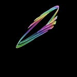
Purple Haze
Even Stranger Attractors
Today I attempted to improve on my previous strange attractor script.
One of the drawbacks of the previous script was the high number of false positives. Thousands of images were being saved to my hard drive but only a few of those were truly strange attractors. The rest were loops, spots, or spiral patterns. I solved this problem by only saving images where at least 1% of the pixels have been visited.
The other drawback was the system of simply painting each visited pixel white directly on an image object, allowing for only a vague silhouette of the strange attractor. A better technique is to record how often each pixel has been visited in an array, and then create an image where the colour of each pixel corresponds to how often it has been visited. This results in much more attractive images reminiscent wispy smoke.


Coming along nicely I think, although more work is needed on the coloring. Source code for this version follows. Note that if you would like to try running this Python script you will need to have both Numpy and Python Imaging Library installed. Also please note that this is not yet the most tidy or efficient code… I’ve left plenty of room for improvement!
import Image
import random
from math import floor
import numpy as np

SIZE = 400

img_index = 0

class Formula(object):
    def __init__(self, seed):
        self.seed = seed
        random.seed(seed)

        self.coefficients = [random.choice([random.random()*4-2,
                        0,
                        1])for x in range(6)]

        self.a, self.b, self.c, self.d, self.e, self.f = tuple(self.coefficients)


    def __call__(self, x, y):

        # return a*(x**2) + b*x*y + c*(y**2) + d*x + e*y + f
        return self.a*(x**2)\
               + self.b*x*y\
               + self.c*(y**2)\
               + self.d*x\
               + self.e*y\
               + self.f

def plotmap(x):
    # scales the x or y up to an integer that fits in our image array

    catchSize = 1

    return int((x+catchSize)*(SIZE/(catchSize*2)))


MAXVAL = 1000

while True:

    random.seed()

    seed = int(random.random() * 10000000)
    f = Formula(seed)

    seed = int(random.random() * 10000000)
    g = Formula(seed)

    x, y = random.random(), random.random()

    imgarray = np.zeros([SIZE, SIZE], int)

    while imgarray[plotmap(x), plotmap(y)] < MAXVAL:

        x, y = f(x, y), g(x, y)
        if not(plotmap(x) and plotmap(y)):
            #print "break"
            break
            # catch negative numbers... the "IndexError" won't
            # do this resulting in "wrap-around" images

        try:
            imgarray[plotmap(x), plotmap(y)] += 1

        except IndexError:
            #print "break!"
            break

    else:
        #print sum(imgarray[imgarray==True].flatten()), SIZE **2
        imgarray = np.array(imgarray / (MAXVAL/256.), np.uint8)

        if sum(imgarray[imgarray==True].flatten()) > (SIZE **2) * .01:
            ## only save image if a certain percentage of the total area
            ## has been coloured.

            img = Image.fromarray(imgarray, "L")
            img.save("a_%06d_%d_%d.png" % (img_index, f.seed, g.seed), "PNG")
            img_index += 1
            print "SAVED!"
Strange Attractors
Lately I’ve experimented with finding strange attractors — A complex mathematical creature generated by a simple repetitive rule. To generate these images, an “x, y” point is first chosen at random and the corresponding pixel is colored white (in a simplified case). Two functions then decide the next “x, y” point:
Which just means that each new x position is determined by some formula incorporating the current x and/or y position, and each new y position is determined by some other formula incorporating the current x and/or y position. Depending on the formulae used, after many thousands of repetitions this may or may not generate an image of a strange attractor.
So it seems that the trick to finding these strange attractors is to simply try out many formulae hoping to generate some interesting patterns. So what formula should I use? According to ThinkQuest, the most common attractor is the quadratic attractor. The formulae used for a quadratic attractor take the general form:

To generate infinite equations of that form I need only tweak the coefficients a, b, c, d, e and f. I can leave out any of the terms (ie. the coefficient can be 0,) or I can leave in a term with no coefficient (ie. a coefficient of 1 is allowed.) For example if I decide on the coefficients 1.4, 0, 1, 2, 1 and -1.2 then the equation will look like:

I put together a Python class to generate these equations:
class Formula(object):
    def __init__(self):
        # generate the random coefficients
        self.coefficients = [random.choice([random.random()*4-2,
                        0,
                        1])for x in range(6)]

    def __call__(self, x, y):
        a, b, c, d, e, f = tuple(self.coefficients)
        return a*(x**2) + b*x*y + c*(y**2) + d*x + e*y + f
This class generates Formula objects which can be called as if they were functions. An example usage would be:
f = Formula()
g = Formula()
newx = f(oldx, oldy)
newy = g(oldx, oldy)
This first attempt is naïve in places but it succeeded in generating the first real results:


Not bad for a first attempt I think. Full Python source follows:
import Image
import random
from math import floor

SIZE = 200 # image size

img_index = 0

class Formula(object):
    def __init__(self):
        self.coefficients = [random.choice([random.random()*4-2,
                        0,
                        1])for x in range(6)]
        #print self.coefficients

    def __call__(self, x, y):
        a, b, c, d, e, f = tuple(self.coefficients)
        return a*(x**2) + b*x*y + c*(y**2) + d*x + e*y + f

while True:

    random.seed()
    seed = int(random.random() * 1000000000)
    random.seed(seed)

    f = Formula()
    g = Formula()

    x, y = random.random(), random.random()

    img = Image.new("RGB", (SIZE, SIZE))

    for i in range(100000):
        #print x, y
        plotx = int(floor(x*SIZE/2))+SIZE/2
        ploty = int(floor(y*SIZE/2))+SIZE/2
        #print plotx, ploty
        try:
            img.putpixel((plotx, ploty), (255, 255, 255))
        except IndexError:
            break
        x, y = f(x, y), g(x, y)

        if not x or not y:
            break # break out of pattern that has diminished to zero

        if x > 1 or x < -1 or y > 1 or y < -1:
            break # break out if growing too big

    else:
        img.save("a_%06d_%d.jpg" % (img_index, seed), "JPEG")
        img_index += 1

